Abstract

Transport mode detection based on mobile phone sensor data is a subdomain of activity detection. State-of-the-art results in literature are usually obtained on limited datasets with few human participants. Approaches used often require ideal situations where sensor data is always available or phones are expected to be in a specific position.

In this article, we discuss a new transport mode classification approach that is trained on thousands of hours of data from thousands of users spread over the world. Our approach can handle missing or low quality sensor data which is important in a production system.

We combine embeddings learned by a convolutional neural network on accelerometer data with a gradient boosting based approach on location information, augmenting the data with an external GIS database.

We show that our late-fusion solution outperforms the state of the art while minimizing memory and cpu requirements, thereby reducing platform cost.

Introduction

Two crucial types of events that make up a person’s day to day journey, are transports and place visits. Whereas place visits might indicate the goal of your trip, the transport mode you choose often correlates strongly with your life stage or way of thinking. Are you a green commuter, a public transport user or a die hard driver?

Thus, a fundamental part of our pipeline at Sentiance starts with transport mode detection. Both Android and IOS already support basic on-device activity detection in real-time, exposing these to mobile developers as ‘motion activities’. However, these API’s yield rather low accuracies and focus on a limited set of transport modes such as walking, biking and vehicle transports, without distinguishing between public transport modes such as train, tram and bus.

We therefore developed our own transport mode detection pipeline that greatly outperforms the current state-of-the-art, both in the wild and in academic literature.

Several vital constraints needed to be satisfied by our solution:

• Low cost: low memory footprint and low cpu requirements
• Edge computing: Can at least partially be deployed on device if desired
• Can be used without accelerometer sensor data, only using location information
• Improves if also accelerometer sensor data is available
• Can cope with real-life situations: gaps in sensor data or bad sensor data
• Multi-modal: can segment trips that consist of multiple different transport modes

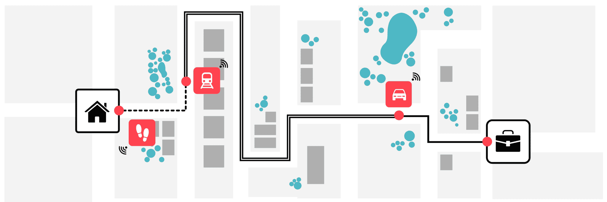
The resulting pipeline is deployed in our cloud based production system and processes millions of trips per day. In the remainder of this article, we discuss each component of the pipeline illustrated by figure 1.

Figure 1. Visual representation of the the multi-modal transport classification pipeline.

It’s all in the vibrations

Every modern smartphone is equipped with an inertial measurement unit (IMU) consisting of at least an accelerometer sensor, often accompanied with a gyroscope sensor.

Accelerometers measure the acceleration, also known as G-force, encountered by the phone in three orthogonal directions as illustrated by figure 2.

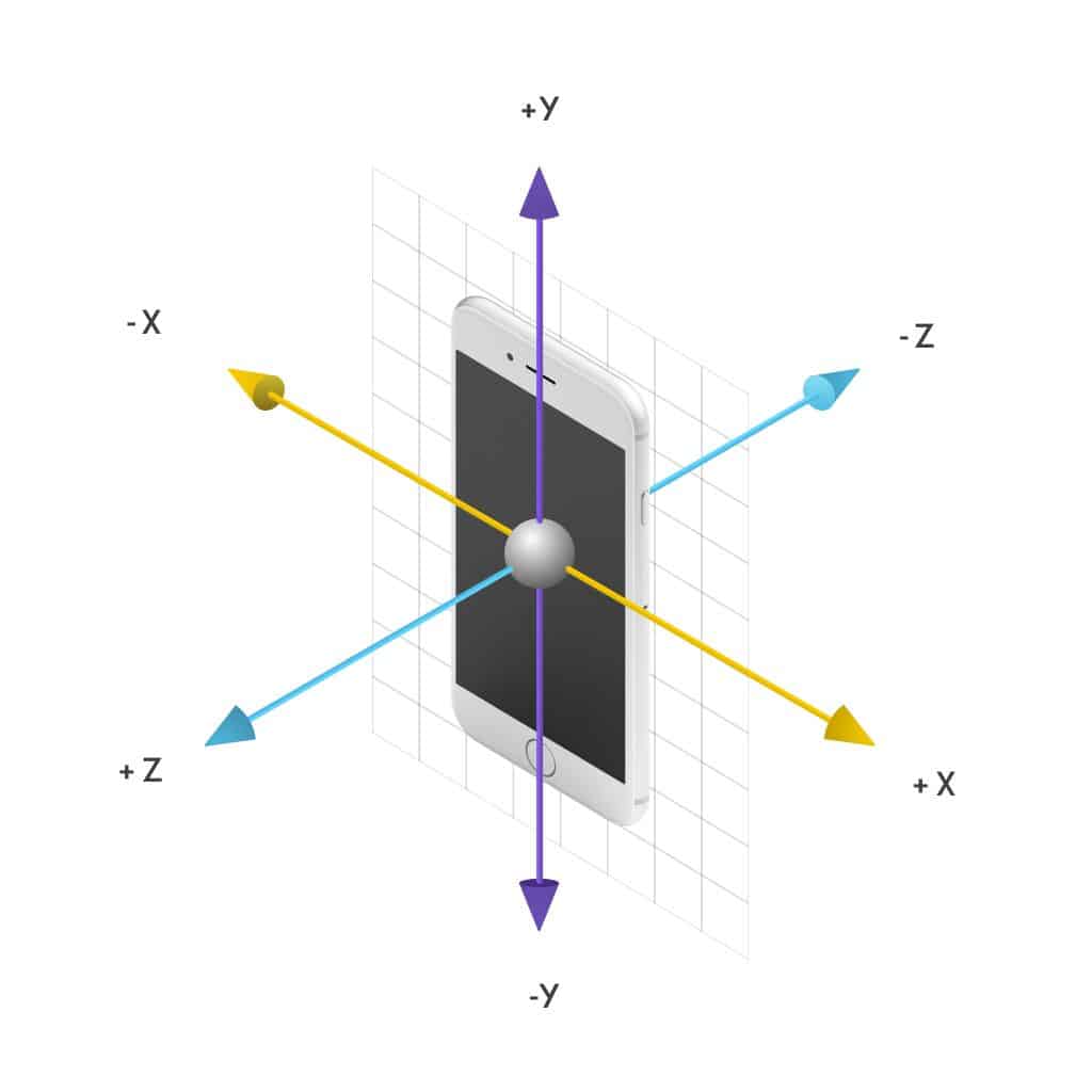
Figure 2. Phone sensors measure acceleration on 3 orthogonal axes.

I These sensors are extremely sensitive, picking up every small vibration of the phone. Figure 3 shows the difference in 3-axes accelerometer and gyroscope data for a trip containing a train segment, a biking segment and a walking segment.

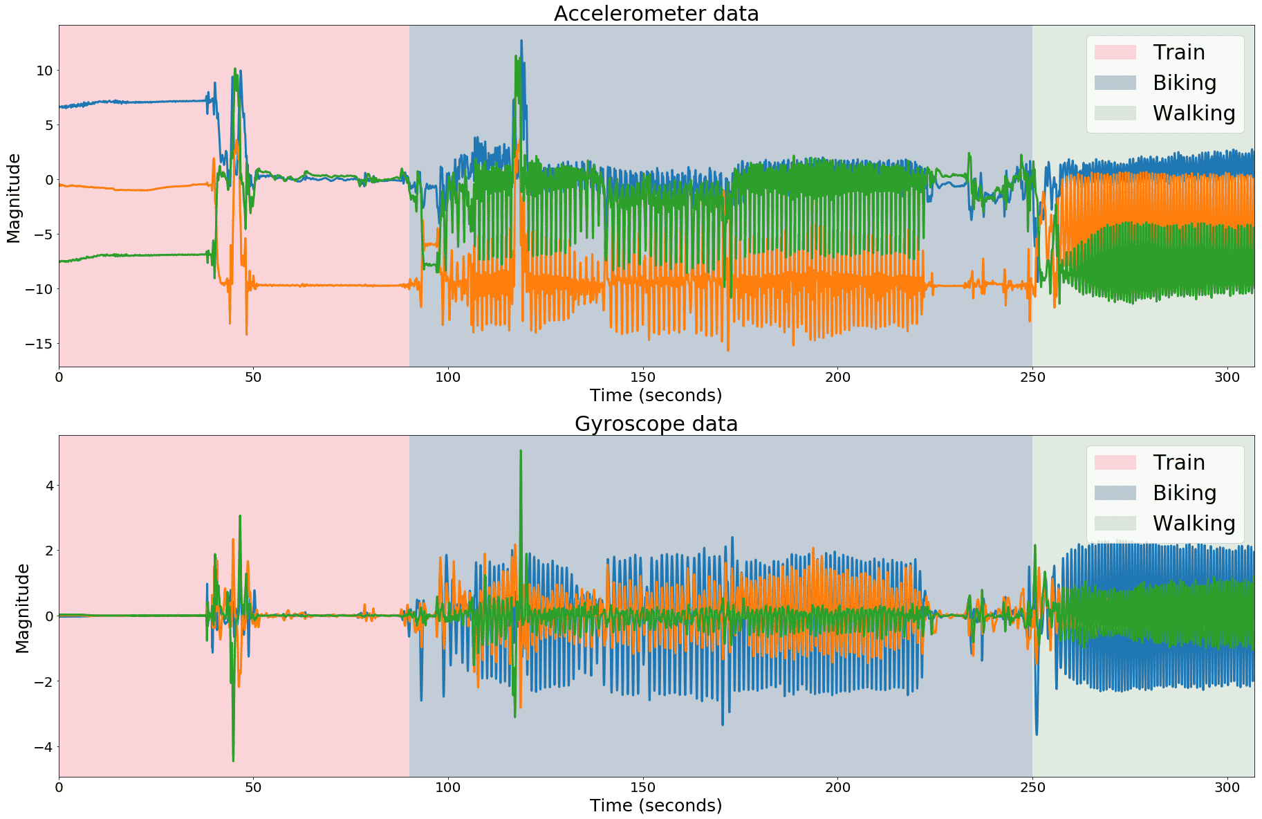
Figure 3. Accelerometer and gyroscope data for a trip containing train, biking and walking segments.

The data corresponding to the walking trip contains a set of low frequency components not present in the train trip. Similarly, car data often contains certain high frequency components that are not present in tram or train data which indicates that frequency domain features would probably be very valuable for activity detection.

This is illustrated more clearly in figure 4, where the frequency spectrum of the accelerometer x-axis of a walking segment (left) is shown, together with the frequency spectrum of a car trip (right).

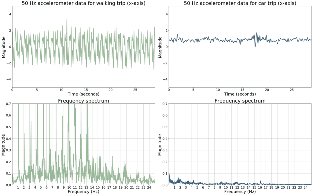
Figure 4. Frequency spectra for accelerometer data from a walking trip (left) and car trip (right).

The walking spectrum shows several high magnitude low-frequency components and harmonics, whereas these are absent in the car data. Similar differences can be observed when comparing spectrograms of biking, train and tram trips, although these differences are much more subtle and difficult to describe with a set of rules or manually engineered features.

Sampling and pre-processing

How can we extract these frequency components, and which sampling rate should be used? Nyquist requires us to sample the data at a sampling rate that is at least twice as large as the highest frequency component we want to be able to extract from the data, which suggests to capture the data at a high sampling rate (e.g. 200 Hz).

On the other hand, battery usage and bandwidth constraints are important factors to consider for mobile applications. Moreover, accelerometer sensors are known to be very sensitive to noise, most of which manifests itself in the high frequency region of the spectrum. For transport mode classification, the importance of frequency components above 13 Hz decreases exponentially. Therefore, we sample the accelerometer sensors at 26Hz.

Although we ask Android and IOS for a 26 Hz signal, we often receive higher frequency data, depending on the phone model and other applications that run on it. Moreover, even for a 26 Hz signal, incoming samples are not evenly spaced every 38.5 milliseconds. We therefore interpolate the signal onto a regular grid, and resample it to get the desired 26 Hz signal.

However, naively downsampling the signal introduces artifacts due to aliasing. Any frequency component above half the sampling frequency would get folded around the Nyquist frequency and incorrectly appear as a lower frequency component in the resulting spectrum.

More concretely, given a sampling frequency fs, an observed frequency in the spectrum can be caused by any real-world frequency component f that satisfies fo = |f - N.fs|, where N is an integer number.

For example, if the original sampling frequency, delivered by the mobile OS, is fs = 36 Hz instead of the requested 26 Hz, then we capture frequency components up to 18 Hz. If we then downsample that signal to 26 Hz, we can only represent frequency components up to 13 Hz. Any component between 13 Hz and 18 Hz however, would now appear as a low frequency artifact in the resampled data.

In this example, a frequency component of 17 Hz in the original 36 Hz signal would appear as a 9 Hz component in the resampled signal, thereby invalidating the true 9 Hz frequency component in the spectrum. This is illustrated with a synthetic example in figure 5, where a 17 Hz sine wave is modulated upon a 3 Hz carrier signal.

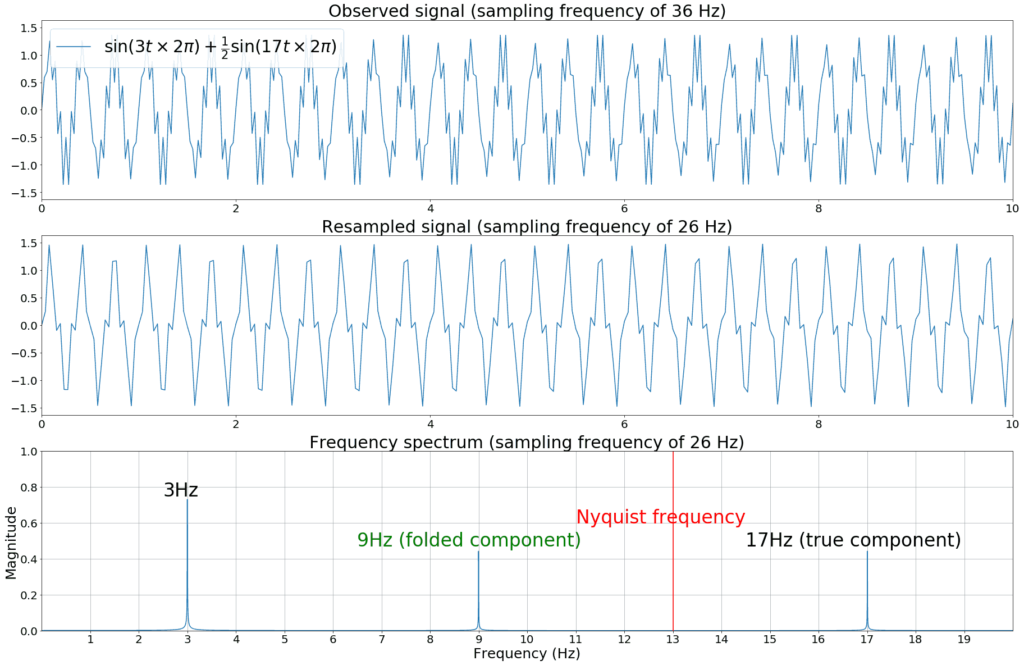
Figure 5. Illustration of aliasing: High frequency components get folded around the Nyquist frequency to low frequency components.

Since the actual sampling rate depends on the mobile operating system and does not necessarily correspond to 26 Hz exactly, we remove these artifacts by applying a low pass filter with a cut-off frequency (-3dB point) of 13 Hz to the signal before resampling.

Another source of unwanted signal components is the gravity pull that directly influences accelerometer measurements. A perfectly still and horizontally aligned phone will show an accelerometer measurement of 9.81 on its Z-axis. Once the phone is tilted, this gravity pull affects multiple axes simultaneously, mixing together with and masking the magnitude of the actual accelerations.

However, phone orientation changes and the corresponding changes in gravity pull manifest themselves as low frequency components in the signal, which in general contain little or no discriminative power for the transport mode classifier. In the extreme case of no phone orientation change at all, the gravity pull would simply appear as a DC offset in the resulting spectrum. We therefore roughly remove the gravity component by simply applying a high-pass filter to the signal with a cut-off frequency of 0.2Hz.
For efficiency reasons, the low-pass and high-pass filters are combined into a single band-pass IIR filter. This is illustrated by figure 6 which shows a 10-second walking segment before and after bandpass filtering.

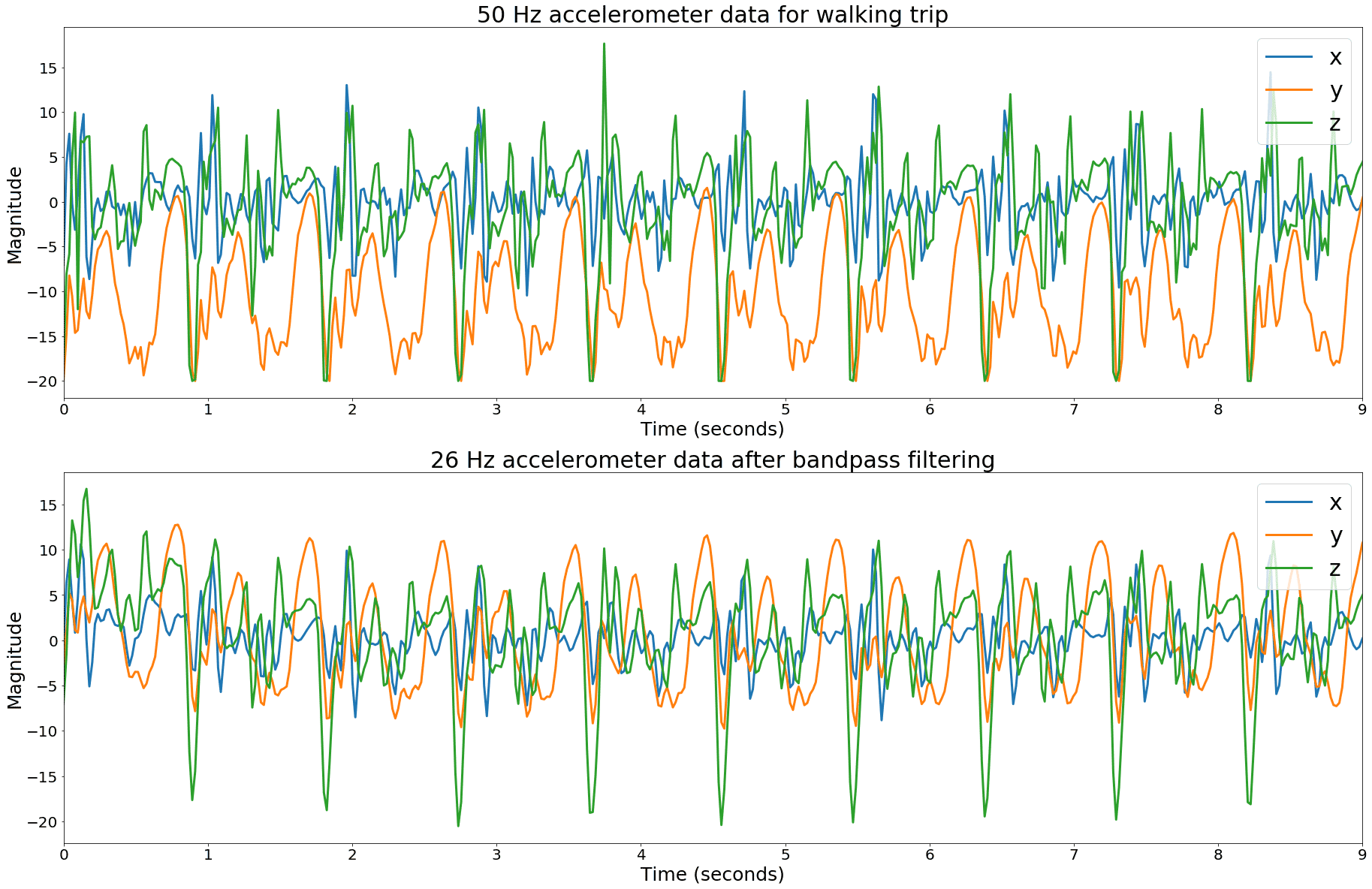
Figure 6. Accelerometer data before and after band-pass filtering to remove low and high frequency components from the data.

Feature extraction and classification

An initial version of our transport classifier depended on a large set of carefully engineered features, both in the time domain and the frequency domain, which were fed into a tree based ensemble classifier. Each window of several seconds of sensor data was described by a set of Fourier coefficients, Cepstrum coefficient, spectral flux, signal energy, zero crossings, variance, etc.

These features were calculated on both the accelerometer data and the gyroscope data. Although the resulting classifier yielded state of the art results, the manual feature engineering process required a lot of signal processing and domain knowledge and was difficult to maintain. Furthermore, we eventually stopped getting further performance improvements, no matter which cleverly engineered new feature was added or what amount of labeled data we added to our dataset.

Given the major advances in applying deep learning to the signal processing domain, i.e. image and audio processing, we therefore replaced our manual feature engineering pipeline with a deep learning based approach.

Surprisingly, we found that our neural network quickly outperformed our original approach, even when trained on only accelerometer data as opposed to also including gyroscope data. Given the fact that many low-end phones lack gyroscope sensors, this allowed us to simplify our complete processing pipeline and to decrease bandwidth and battery requirements of our mobile SDK even further.

Moreover, whereas our manually engineered features seemed to be most descriptive when using short, five second windows of sensor data, the convolutional neural network is able to extract more meaningful information from longer sensor windows up to 30 seconds. Longer windows basically allow the bottom layers of the network to learn filters with a frequency response of much higher resolution compared to those learned from smaller windows.

Convolutional neural network with weight normalization

We trained a simple 7-layer convolutional neural network with dropout and some max pooling layers. We played around with popular regularization techniques such as batch normalization and L2-norm, and with different optimizers such as Adam and RMSprop. Eventually, we settled for stochastic gradient descent with Nestrov momentum, and weight normalization, which greatly sped up convergence during optimization.

The network was trained for 25 epochs with a batch size of 256. Each sample consisted of a 24 seconds accelerometer window, represented by 624 data points. These windows are extracted from more than 2000 hours of carefully labeled sensor data. A stride of 9 seconds was used, yielding 5 transport mode detections per minute which are aggregated into a per-minute transport label later on.

Figure 7 shows our network architecture, which we implemented using Keras and Tensorflow and deployed as a microservice in our Kafka based reactive architecture.

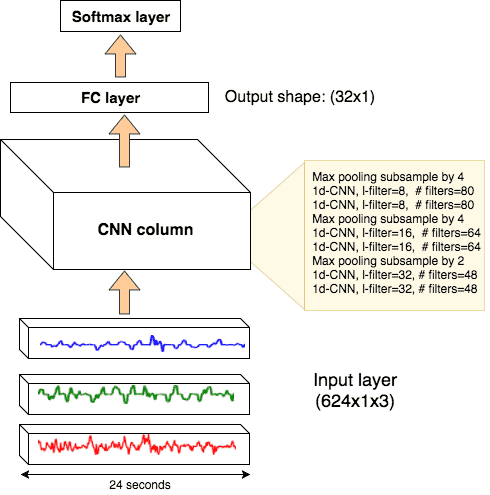
Figure 7. Visual depiction of our Neural Network architecture

Note that the limited number of parameters used makes it possible to deploy this model on the mobile device itself, opening up further opportunities to reduce cost and improve real-time characteristics.

Data augmentation

Our datasets contains more than 2000 hours of carefully annotated sensor data, representing real-life transports in different parts of the world. This corresponds to more than 276,923 labeled 26-second sensor windows.

To further increase our dataset size, we heavily make use of data augmentation. This greatly improves generalization capabilities of the classifier to different phone orientations and contextual situations (e.g. the phone can be mounted to the windshield, tucked away into the user’s pocket, placed into a cup holder, etc.).

Simulating different phone orientations can be accomplished easily by rotating the 3D data around one or more of the X, Y or Z axes. For each labelled trip, we randomly select three angles between 0° and 180°, create a 3D rotation matrix, and apply this transformation to the sensor data. The augmented trip is added to our dataset and the procedure is repeated several times.

This is illustrated in figure 8, and effectively forces our network to learn feature representations that are invariant to the phone’s orientation and removes the need to estimate linear acceleration using error prone attitude estimation techniques such as extended Kalman filtering.

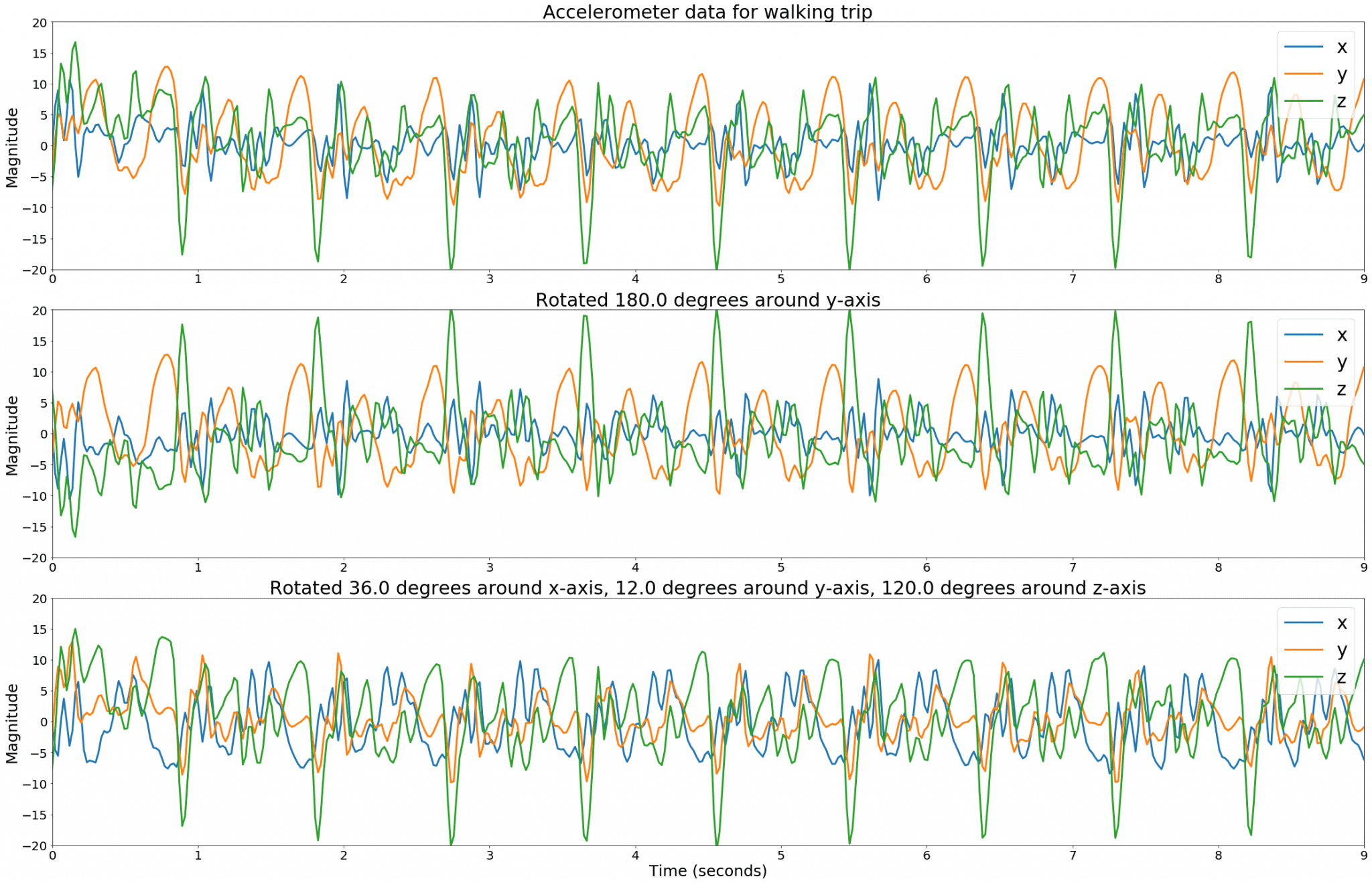
Figure 8. Accelerometer data after rotating in 3D to simulate different phone orientations.

A second type of data augmentation we use is data obfuscation to make sure the classifier does not learn device or user specific features. Due to manufacturing imperfections, each phone exhibits slightly different noise characteristics which can be used to fingerprint devices and identify users. Since we want our classifier to learn to identify transport modes instead of learning to remember which transport mode specific users prefer, we therefore obfuscate the sensor signal.

This is accomplished by adding additive and multiplicative noise. Since white noise corresponds to a flat frequency spectrum, this is an easy way of masking out device specific characteristics without significantly altering the spectral envelope of the signal.

After data augmentation, we end up with a dataset of approximately six million labeled windows.

Results

We divided our training data in a training set, a validation set for model selection and hyperparameter tuning, and a test set to report final accuracies on as shown below:

Note that we also detect bus and running as post-processing steps:

1. Running is detected with high accuracy by applying a simple linear model on transports that were detected as walking
2. The transport classifier initially reports ‘bus’ trips as ‘car’. To further split up this class, we then trained a model using our ‘deep driver DNA embeddings’ as input features. Based on the user’s driving behavior, the model is able to accurately separate bus trips from car trips.

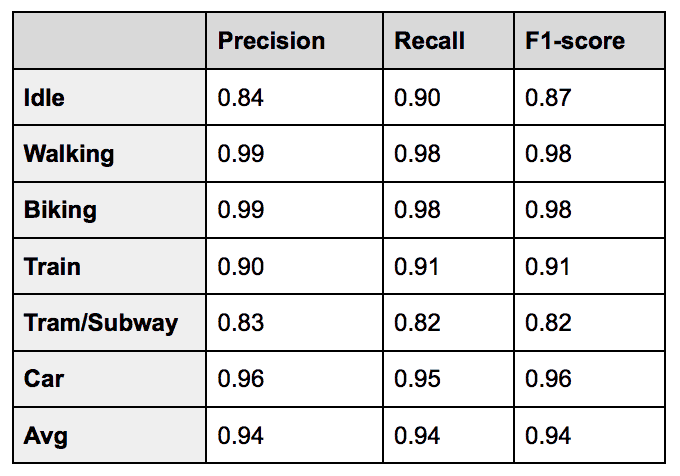
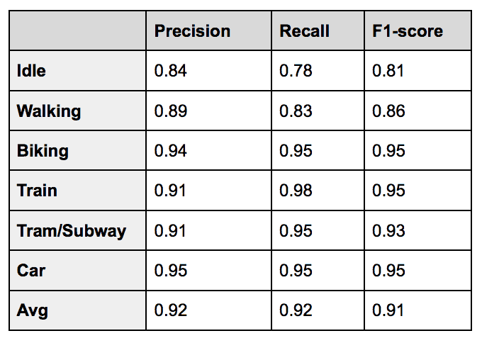
Clearly the classifier has no problems distinguishing walking and biking from vehicle transports, but struggles somewhat when presented with tram or train trips or with idle segments. The reason for this is that modern railway vehicles tend to drive very smoothly, limiting the amount of information that is available in the frequency spectrum of the signal. This is illustrated in figure 9, which compares car data containing an idle segment, with tram data containing no idle segment.

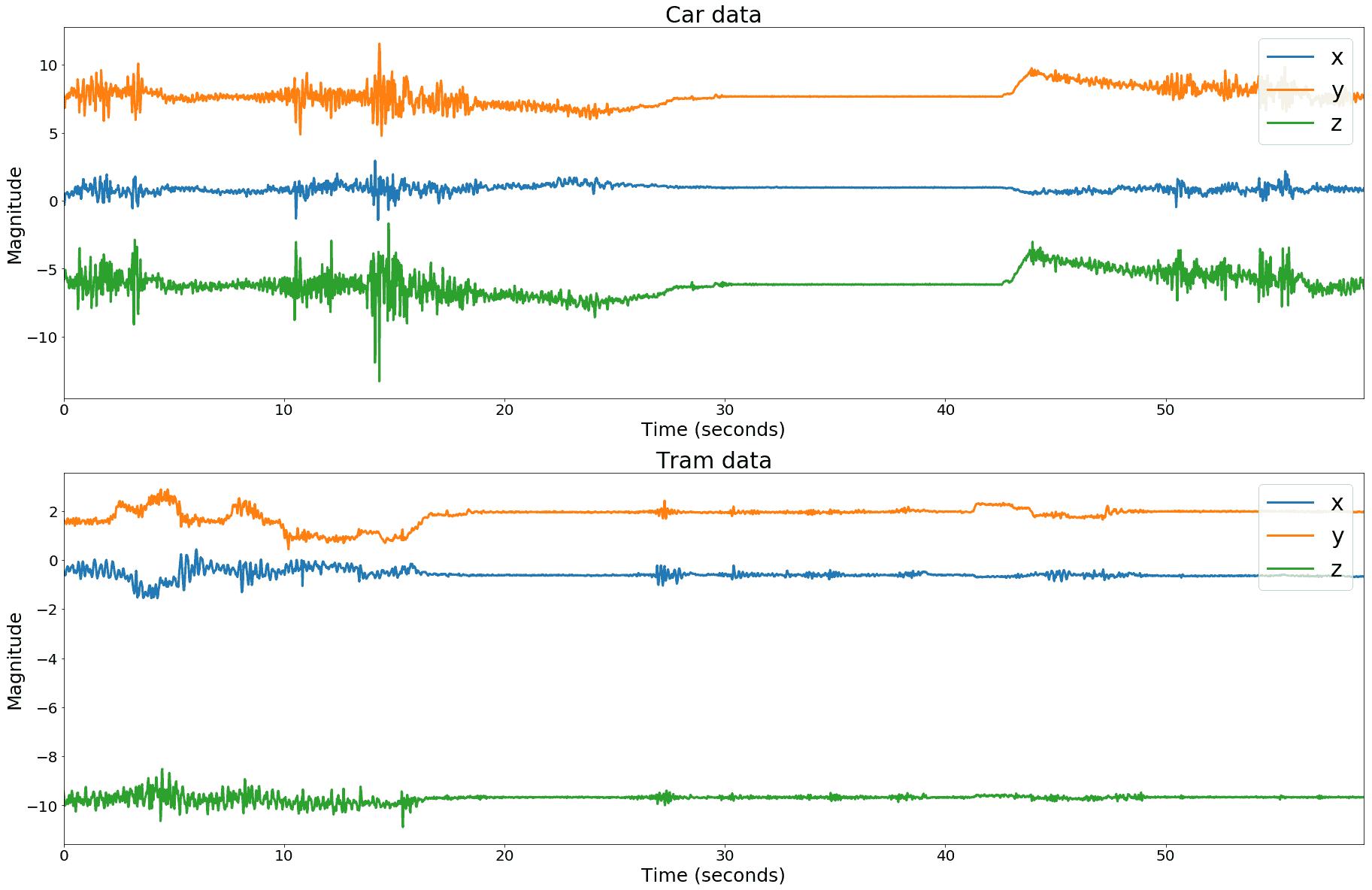
Figure 9. Idle segments in car trips look very similar to non-idle segments in tram or train trips.

Although the presented results outperform what is available in academic literature while being trained and tested on a much larger dataset, they are clearly not adequate for a production system without further steps. A recall of 82% for tram means that almost one in five tram trips is misclassified. Moreover, a precision of 83% means that almost one in five transports is incorrectly considered to be tram.

However, if we chop off the top layer of the CNN and keep the last fully connected layer, we now have a 32 dimensional embedding space that captures sensor specific transport features, which we can combine with other information to make a final decision.

An important feature that we neglected in the previous discussion, is location information and its derivatives such as speed. In the next paragraph, we discuss a transport mode classification approach that only considers location based information in order to illustrate that both data sources are highly complementary. In the last paragraph of this article, we will then combine our sensor based embeddings with the location based classification results in a late fusion fashion to obtain a highly accurate multi-modal transport classifier.

Location context says it all

To avoid a noticeable battery drain, our SDK currently requests a location fix from the operating system approximately once per minute. The location fixes reported by Android and IOS fuse GPS, WIFI fingerprinting and cell-tower information together, and use some internal heuristics to estimate a measure of accuracy.

In the following paragraphs, we discuss a simple classifier that estimates the transport mode for each waypoint. Compared to the sensor based classifier, this location based approach obviously yields a much lower temporal resolution.

Although a location fix is requested once per minute, we often receive much less location information, especially when the user is transporting in urban canyons where signals reflect off or are completely blocked by big buildings, or when traveling at high speed in vehicles that tend to behave like Faraday cages. Thus, location-only based classification can be used as an indicator of transport mode, but is often not sufficient for mobility applications where accurate temporal segmentation is mandatory.

Feature extraction

Figure 10 shows some location fixes received from the mobile phone during a car trip (left) and a train trip (right).

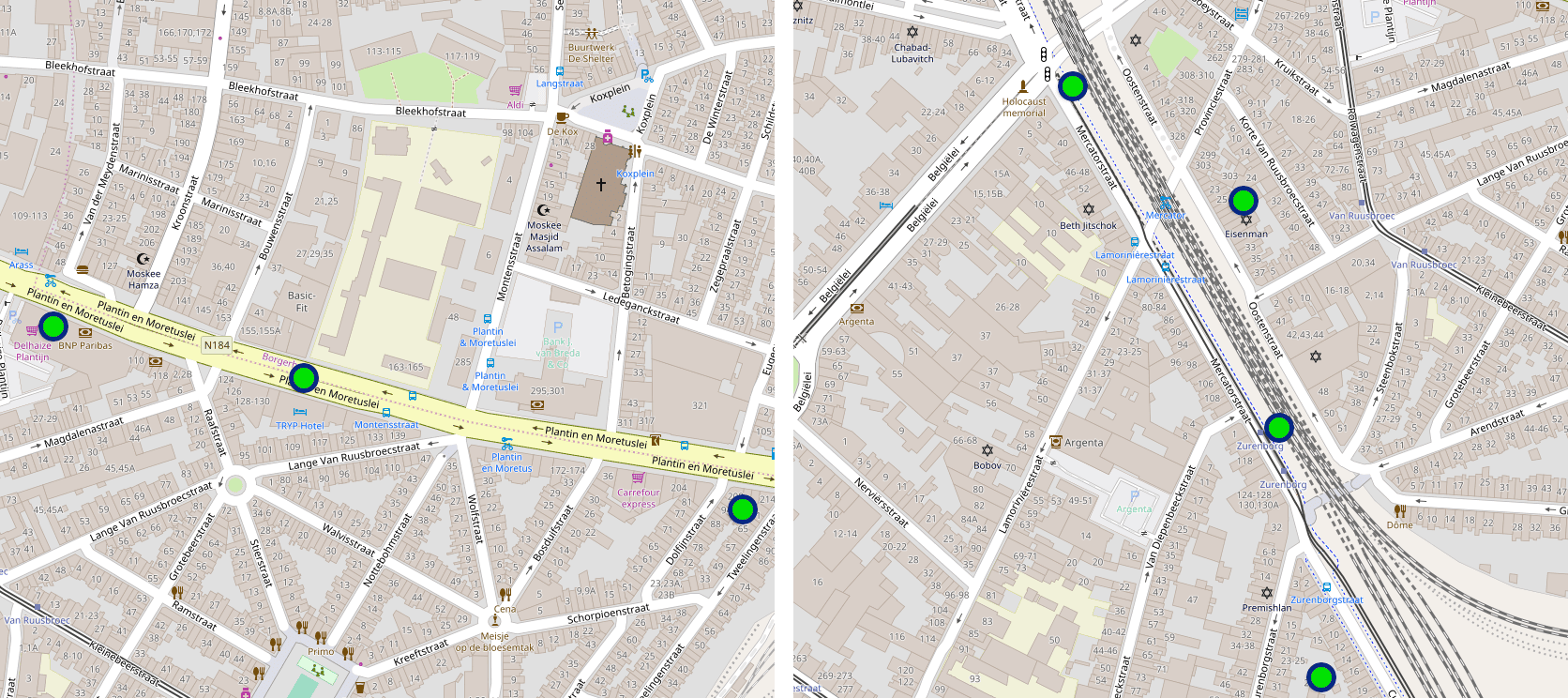
Figure 10. Waypoints for a car trip (left) and a train trip (right) illustrating the importance of contextual GIS data.

Without looking at the sensor data, and even without any information about speed and duration, one can easily deduce the transport mode by simply looking at the map and road network.

Thus, as part of our feature engineering effort, we query our GIS (Geographic Information System) database - a local copy of the Openstreetmap planet data - to get distance estimates to railroads, highways, pedestrian roads, tram stops, etc.

This feature vector is further augmented using velocity information, as speed of travel is an obvious indicator of transport mode, and with some spatial information such as distances between subsequent location fixes.

Finally, for each waypoint we add the k-nearest (in time) motion activities as reported by Android and IOS in a simple one-hot encoded manner as additional features. These motion activities are noisy and often inaccurate, but represent a cheap source of sensor based information that at least correlates with the correct transport mode on average.

Classification

Each 24-second time window is represented by the concatenation of the feature vectors of the two nearest (in time) location fixes. This allows the classifier to learn some short-term temporal dependencies and to smooth out its predictions.

We trained a gradient boosting classifier with decision trees as its base learners using XGboost, and use a grid search on a hold-out validation set to optimize the hyperparameters. The following table illustrates the 10-fold cross validation results:

Whereas the sensor based classifier had difficulties distinguishing train from tram, the location based classifier seems to have trouble distinguishing walking from biking. Including GIS based features such as distance to highways, railroads or tram stops seems to improve vehicle based classification accuracy rather significantly, while trajectories and speeds for walking and biking trips are often very similar, leading to confusion between those classes. Moreover, due to the limited granularity in time, the location based classifier has difficulties detecting idle segments that are usually very short.

Ensembling to the rescue

Given the highly decorrelated classification results of the sensor based classifier and the location based classifier, both predictors could be combined in an ensemble, reducing the bias and the variance of the final classification by cancelling out each other’s mistakes.

However, the softmax layer of the sensor based classifier potentially throws away useful information while linearly combining the activations from the preceding fully connected layer into a lower dimensional vector. Instead of using the output class probabilities directly, we therefore simply chop off the top layer of the neural network, and use the 32 dimensional feature space of the dense layer as a feature vector instead.

This 32D embedding is combined with the 6D vector representing the class probabilities of the location based classifier by concatenating them into a single feature vector. The resulting feature vector contains a rich and targeted representation of both low level sensor based features and high level GIS based information for every part of the trip.

The following video shows a 3D projection of our 38 dimensional feature space, obtained using t-SNE.

Since the different transport modes are almost linearly separable in this feature space, we trained a logistic regression classifier on a third hold-out part of the dataset that was never seen by either the sensor based classifier or the location based classifier. Results are shown below:

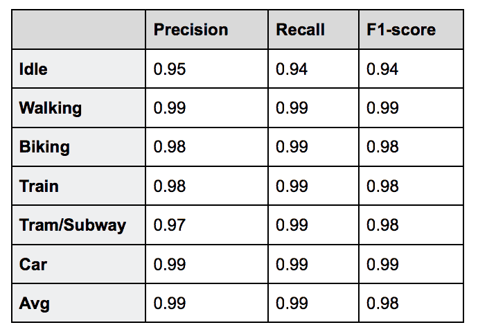
As expected, the final classifier outperforms both individual classifiers. Moreover, applying a late fusion method like this allows us to distribute the computational load by deploying part of the model on-device while doing the rest of the computations in the cloud.

Finally, for specific customers where battery usage and bandwidth constraints or of extreme importance, we can easily fall back to one of the individual classifiers such as the location-only based version directly.

Performance and cost

Apart from the accuracy gain, converting our random forest based sensor classifier to a deep learning based approach yielded a significant reduction in platform cost.

The original random forest based approach required some heavy signal processing to obtain a set of features, many of which appeared to be not sufficiently descriptive to obtain the highest quality results. The neural network on the other hand, learns to extract only those features that contribute to the goal of classification, which greatly reduces computational complexity.

Moreover, the original random forest contained thousands of trees and millions of parameters, resulting in models with huge memory requirements. The neural network on the other hand only contains a few hundred of thousands of parameters, easily fitting in memory, both in our cloud based backend or on the mobile device itself.

Figure 11 shows classification times for both the original classifier and our deep learning based solution.

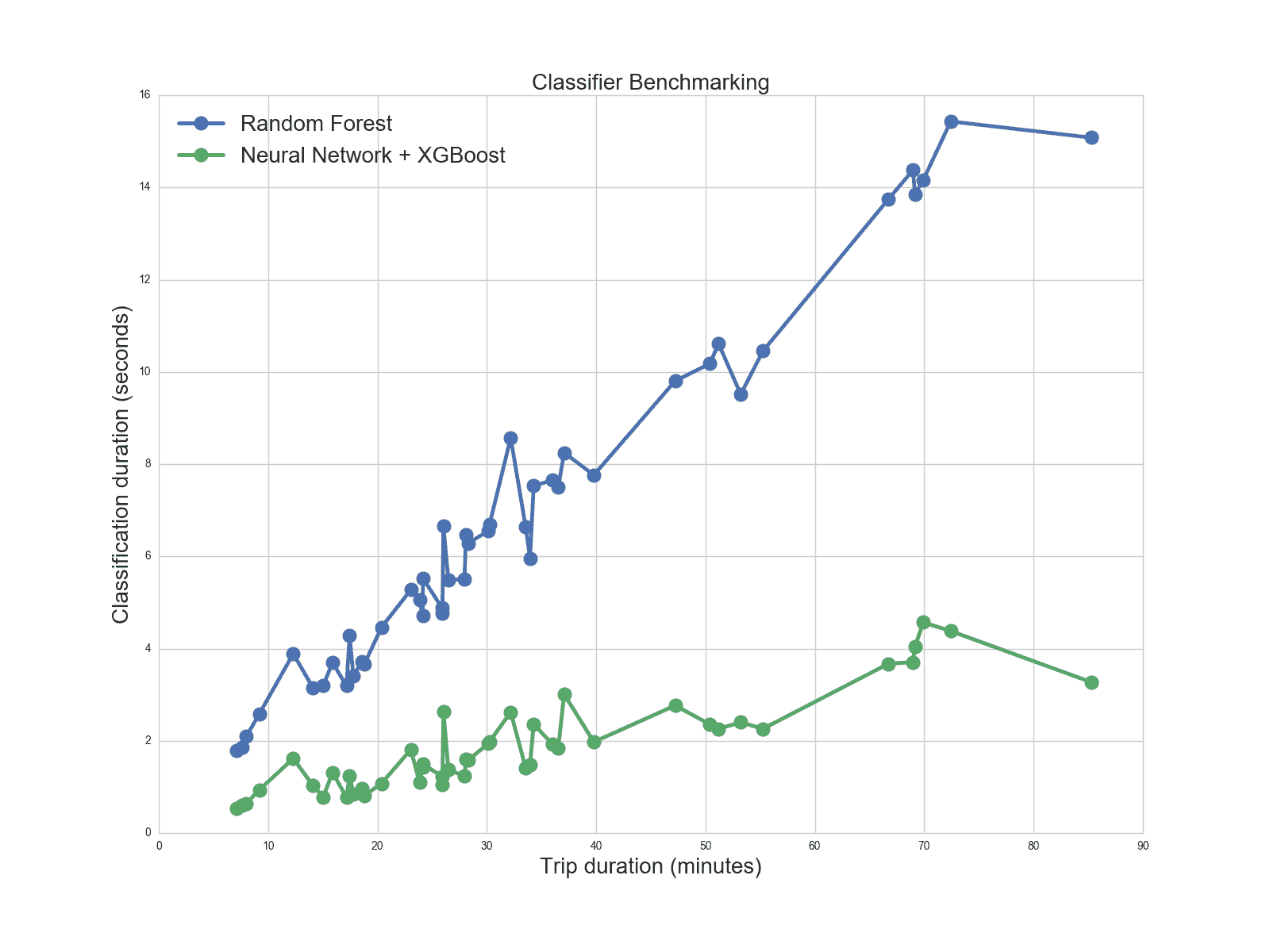
Figure 11. Classification duration relative to trip length

This indicates as 4-5x improvement in throughput, which results in a giant cost reduction as our back-end receives several millions of trips per day.

Conclusion

In this article, we showed how we perform transport mode classification at Sentiance, and how we support both those uses cases where accuracy is paramount and low level sensor data can be used, and those where cost and battery consumption is more important thus resorting to only location information.

Our solution is being used in many different verticals, ranging from lifestyle coaching in the health sector, to driving behavior modeling and fleet tracking in the insurance and mobility space. Given the different needs and constraints of these verticals, we constantly need to balance accuracy, speed, battery drain and cost.

If you want to know more about the rest of our product, or are eager to test our accuracies yourself, download our demo app Journeys!

Retweet this article!