Sentiance provides a cutting-edge driving behaviour scoring technology. Based on sensor data collected from the user’s mobile phone we compute scores characterizing smooth driving, anticipative behavior, compliance with speed limits and focused driving. However, not every car trip should be aggregated into the user profile. Being a passenger of a reckless taxi driver shouldn’t penalize your driving profile. In this blog post, we will describe an approach to detect whether a person in a car is the driver or a passenger using solely the low-level sensor data.

Driver DNA

We first introduce the concept of driver DNA: a unique driving behavior profile, a fingerprint that is specific only to that driver. In order to derive that driver DNA, we first need to extract meaningful features from individual car trips. Later on, we aggregate features over many trips to derive a general driving profile. The source of the data is the mobile phone’s accelerometer and gyroscope sensors.

From the raw signal, we derive the longitudinal and lateral accelerations of the car as well as its yaw or angular velocity in the vertical axis (Fig. 1). Sentiance has state-of-the-art attitude estimation technology to compute the accelerations and angular velocity in the referential of the car in which a phone is placed in an arbitrary position (find out more in this blog post).

The signals from Fig. 1 capture patterns that relate to how a person drives. On the same road, for a given situation in traffic, an aggressive driver generates big peaks in the acceleration while a smooth driver doesn’t.

Other factors than the driver DNA affect the sensor response too. Different roads will result in different turn patterns: driving up a curvy mountain road generate different data than cruising on a highway. Also, for the same road and driver, traffic will influence the acceleration and braking distributions. We therefore need a model that is able to characterize driving profile, independently of the road type, traffic, and car type.

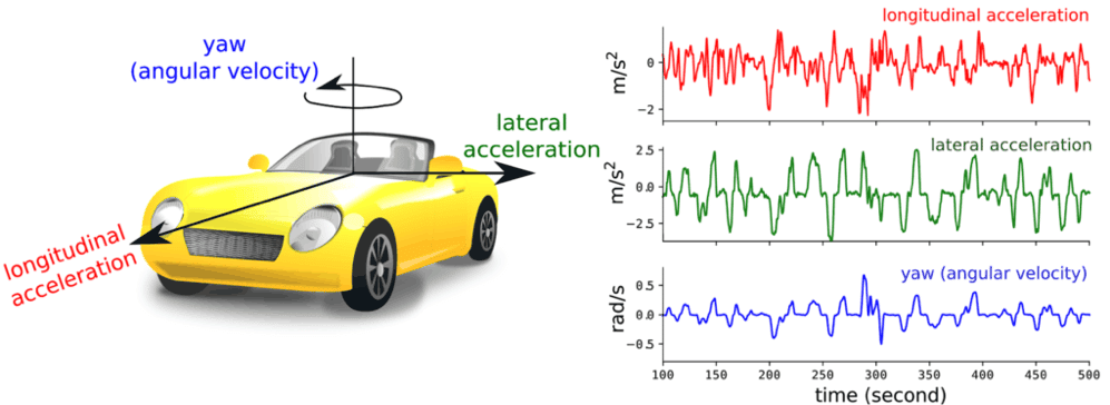
Figure 1: from the sensor data collected on a mobile phone present a car, we derive the longitudinal and lateral acceleration of the car as well as its yaw.

Different driving styles result in different signals, and an efficient encoding thereof will yield features that can differentiate between drivers. One could choose to manually engineer features, taking for instance signal statistics or wavelet coefficients.

While such an approach has proven useful in speech or music processing, where we intuitively know that features such as modulation frequency convey information about the sound object, nobody knows what features are important when characterizing driving behavior.

We therefore decided to tackle this problem using a deep learning (DL) approach. In DL the feature extraction stage is part of the neural network: if a feature is important to solve the task of interest, the network will learn to extract it.

Elementary driving events are single accelerations, brakes, or turns, which have an average time scale of a few seconds. The temporal interactions between those driving events also contain a lot of information about our driving style: how fast does one change gears, how hard does one brake before a turn, how smooth do you go to cruising speed, are all part of our driver DNA and are reflected in the sensor data.

Nevertheless, we assume that this temporal interaction shouldn’t be considered in a time window larger than 30 seconds. Indeed, longer patterns will very likely be mainly characterizing the road layout rather than the individual driving style.

Deep feature extraction

As data manual labeling is a tedious and expensive process, we don’t have thousands of hours of car trips tagged as either driver or passenger. Nevertheless, during the last couple of years, we collected hundreds of thousands of hours of sensor data from car transports from many users.

Therefore, instead of directly learning to distinguish between drivers and passengers, we learn a user-specific embedding: the driver DNA.

Inspired by transfer learning literature, we trained a network using a simple softmax output layer such that it learns to recognize which userID a trip originates from. We then assume that one of the top layers of the network learned a high-level representation of user-specific driving behavior. Trips in which a similar driving behavior is apparent should be close to each other in the learned metric space, whereas trips with a different driving behavior should be far apart.

Chopping off the softmax layer and using one of the last dense layers as our feature space, we, therefore, obtain a feature vector that characterizes the driver DNA of a trip segment.

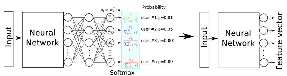
Figure 2: the network is trained for classification on user ID. The last dense layer is chopped off leaving the second last layer which becomes our output feature layer.

The network that learns this feature space operates on 30-second long sensor segments. The first layers should encode the elementary patterns on a short time scale, whereas the subsequent layer should account for the temporal relationship between those patterns. We therefore use a Convolutional Neural Network (CNN) with an LSTM layer stacked upon.

CNNs are a popular choice for representation learning. They learn gradually more complex filters sensitive to patterns relevant to the task learned.  LSTM is nowadays the standard choice to encode sequences, for instance in language translation.

The input to the CNN column is a tensor of length 128 (+- 30 seconds) and depth 3, containing lateral and longitudinal acceleration and yaw (gyroscope), as illustrated in figure 3. The CNN column consists of 12 1-dimensional (time-axis) convolutional layers. Each layer has a leaky ReLU activation function followed by batch normalization. Layers are functionally divided into groups where the field of view, i.e. filter length, increases. Max pooling between these groups reduces the length of the time axis from 128 to 16.

The output vector of the CNN can thus be seen as a compressed encoding of the 128 time steps of the input signal into only 16 time steps. To further model temporal dependencies between these 16 time steps, the output of the CNN is passed to an LSTM layer.

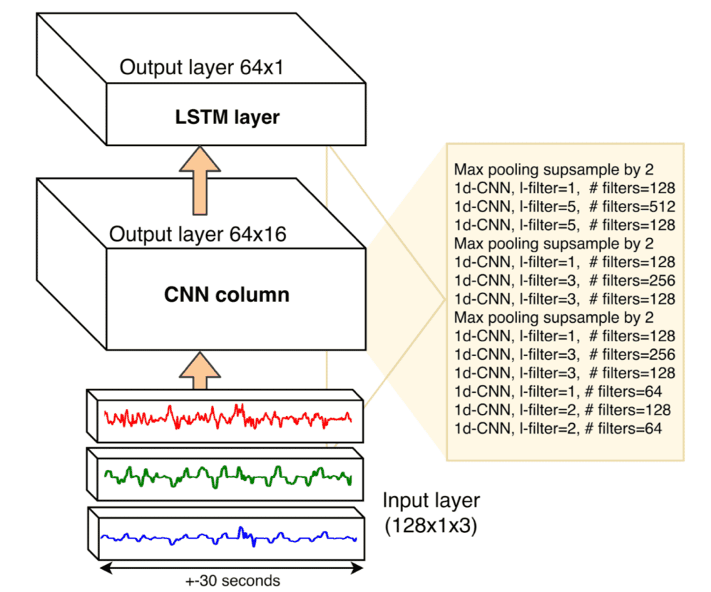
Figure 3: architecture of one neural column

While our input window length is 30 seconds, a normal car trip is much longer. To integrate features from consecutive windows, we apply the neural column from Fig. 3 to subsequent 30-second windows of the same trips with 25% overlap (Fig. 4). The input to the network is therefore a 4-minute long segment.

As we want to learn the same patterns at each 30s segment, the neural column for each 30s window is the same. The output of each column is fed to a layer that averages the features of the different windows. The averaging layer feeds into a two-layer dense network with 20% of dropout (80% of the connection are kept) which in turn inputs to a softmax layer. The whole network contains about 2M trainable parameters.

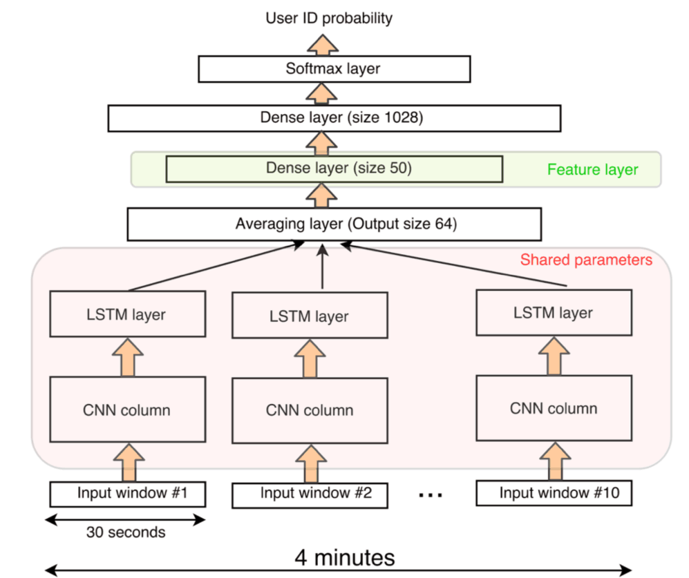
Figure 4: the same neural column encodes different input windows. Their output is averaged then fed to a 2-layer dense network. After the network is trained, the output of the first dense layer is the driver DNA  feature layer.

The network was trained using Keras on an AWS GPU machine. We used the Adam optimizer with a categorical cross-entropy loss.

Different data augmentation schemes were implemented in a batch generator:

1. Turning left or right should be considered equivalent, so the lateral acceleration and gyroscope signals were sign-reversed
2. Small amount of white Gaussian noise was added to all signals to diminish device-specific noise characteristics
3. Signals were slightly scaled by Gaussian multiplicative noise, to further diminish device-specific noise characteristics

The best  top-5 validation accuracy was 79% percent. Very high generalization might not be possible on this dataset because of inherent noise in the labels. Indeed, for a given user, the data is corrupted with trips misclassified as a car or when the user was actually a passenger. Furthermore, we are not interested in the user classification per se but in extracting a feature vector from each trip segment. In Fig. 5 we can see a t-SNE 2D projection of the feature layer vectors from trip segments of three users of the validation set. As expected the activation patterns at the second last layer allow for the discrimination of user driving profiles.

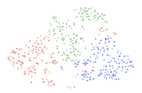
Figure 5: t-SNE 2D projection of trip segments from three users from the validation set. Each color corresponds to a user.

Driver-passenger classification

To test different strategies to detect passenger trips, we collected labeled data from Sentiance employees. During three months they were asked to annotate all their car trips as either ‘driver’ or ‘passenger’.

Sentiance users and trips were not part of our training set. After running our trained model on all the trips of a given user we can project the feature vectors onto a 2D space using t-SNE (Fig. 6) While the driver segments (blue dots) cover most of the distribution, the passenger segments (red dots) are confined and clustered at the edge. Thus, to separate driver trips from passenger trips, we can cast our problem into an anomaly detection problem in our learned feature space.

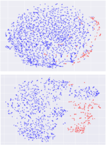
Figure 6: t-SNE 2D projection of trip segments. Upper and lower plots correspond to two different users. The blue dots correspond to driver trips and the red ones to passenger trips. Passenger trips are clustered and confined at the edge of the trip distribution.

Anomaly detection

We first make the assumption that, in most of the cases, the user is the driver of the car. We cast the problem as an outlier detection: if the driving behavior during a trip is very different than most of the trips seen before for that user, the trip is classified as passenger. One advantage of this approach is that it doesn’t assume the sample we collect has only positive labels i.e. that they are all driver trips. As long as the passenger trips do not happen too often the main modes of the distribution will correspond to driver trips with high probability.

We use the isolation forest (IF) algorithm (F. Liu et al 2008). The IF is trained on the 50-dimensional driver DNA features from many trips from a user (Fig. 7).  At the inference stage, it returns regularity scores for each segment, that are then averaged on the trip level. If the average trip score is below a predefined threshold, it is labeled as passenger, otherwise as driver. The threshold is estimated using a condition on the second derivative of the score probability distribution.

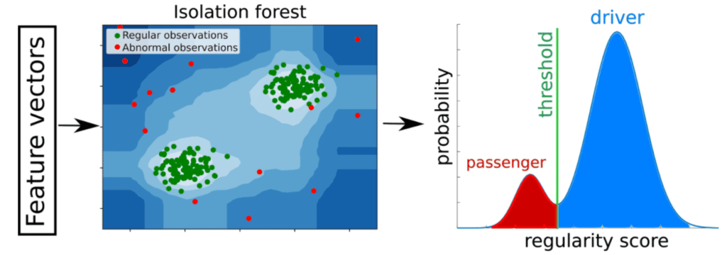
Figure 7: concept behind the anomaly detection approach (2 dimensional vectors are shown for the sake of visualization but in reality the vectors have 50 dimensions). Regular patterns result in high regularity scores whereas abnormal one are given low scores. The score distribution for the population is estimated and a threshold defines the boundary between passenger and driver trips.

In Fig. 8 we can see the results for a user with ground truth data. The passenger trips clearly receive lower regularity scores than the driver trips. The area under the curve (AUC) of the receiver operating characteristic (ROC) curve is 0.94. If we fix the threshold using our heuristic method, the classification power can be summarized using different metrics (see table). As the dataset is unbalanced we also report the Matthews correlation coefficient (MCC). It takes into account true and false positives and negatives.

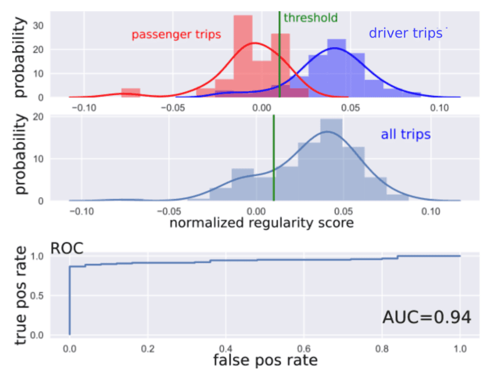
Figure 8: results for a user with ground truth data using the isolation forest. First row: the probability distributions for the passenger trips (in red) and the driver trips (in blue). The decision threshold is shown in green. Note that the histogram are normalized with respect to the corresponding distribution. Second row: probability distribution of all trips. The threshold is estimated from this distribution, i.e. the one where we don’t know the label of the trips.

Universal model

A potential disadvantage of the isolation forest approach, is the need for rather large amounts of trips before the user’s driver DNA can be modeled.

Inspired by user identification and biometrics literature, in which the user of a system is either granted or refused access based on their recent behavior, we therefore implemented a second approach where driver-passenger classification is cast into a driver identification problem (driver vs rest of the population classification).

We followed the procedure that proved very efficient in speech identification (D. Reynolds et al 2000) and smartphone user identification (N. Neverova et al. 2016), where features are extracted from mobile phone sensor data using recurrent DL networks.

An overview is shown in Fig. 10. We first need a universal background model (UBM): a generative model, a Gaussian Mixture Model (GMM) with 128 components, is trained on the features vectors from the trip segments of our training population. For each new user, a personal model is derived by updating only the mean and weights of each component of the GMM. After having seen enough trips, the user GMM will model the user driving profile.

To tell if a trip is a driver or passenger trip, the average log-likelihoods from the UBM and the user-specific GMM are compared. If the trip was more likely to have been generated by the UBM then the trip is classified as passenger whereas if it was more likely to have been generated by the user GMM then the trip is classified as driver. Again, the threshold is estimated using a condition on the second derivative of the probability distribution of the log likelihood difference.

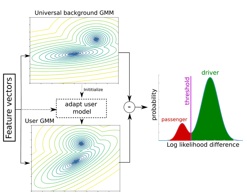
Figure 9: a GMM is trained on the features from the training dataset, resulting in a universal background model (UBM). A new user model is first initialized with the UBM. When car trips arrive for a new user, the UBM is updated and converges to a personalized model. At inference time, the log likelihoods from both models are computed. If the difference is above a predefined threshold, the trip is more likely generated by the user model, and the trip is seen as driver. If the difference is below the threshold, the trip is more likely generated by the UBM and the trip is seen as passenger.

In Fig. 10 we can see the results for a user with ground truth data. On average, passenger trips are more likely to be generated by the universal model. The AUC is 0.88. If we fix the threshold using our heuristic method, the classification power can be summarized using different metrics (see table). In this example MCC=0.66.

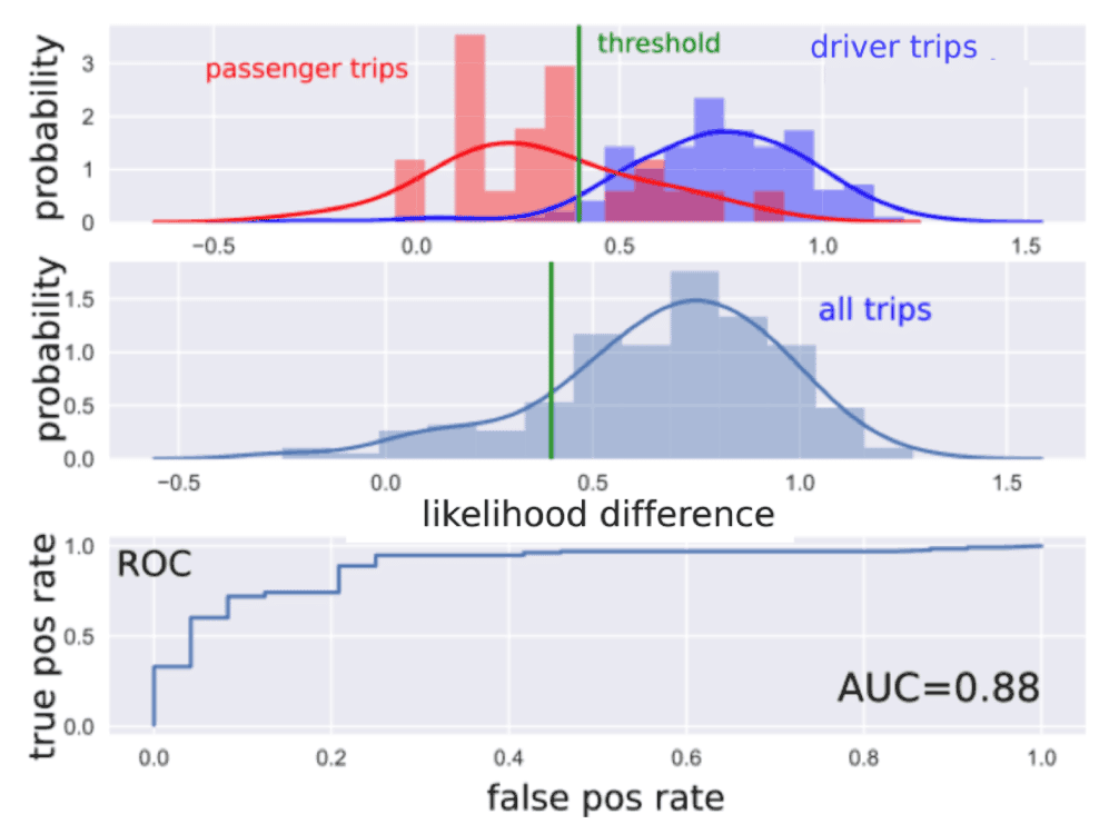
Figure 10: results for a user with ground truth data using gaussian mixture models. First row: the probability distributions of the normalized likelihood difference for the passenger trips (in red) and the driver trips (in blue). The decision threshold is shown in green. Note that the histogram are normalized with respect to the corresponding distribution. Second row: probability distribution of all trips. The threshold is estimated from this distribution, i.e. the one where we don’t know the label of the trips.

Combining both algorithms

For some users the IF algorithm works better than the GMM (like in the two examples) whereas for other users the GMM outperforms IF. This can be due to the number of passenger trips contaminating the training set at the beginning of learning. We decided to combine both approaches: if any of the two algorithms classify the trip as a passenger trip, the trip is classifier as passenger.

Conclusion

In this blog post, we presented how we used deep learning to extract features from car trips in order to detect passenger trips. The approaches work best if the number of passenger trips per user represents a minority of the trips. Indeed, in order to use an isolation forest we must assume that passengers are outliers. Similarly, too many passenger trips would contaminate the adaptation of the user’s gaussian mixture model. If that assumption holds, we are able to reach a precision of 0.73 and a recall of 0.76 on average for the passenger trips and an average total accuracy of 0.91.

We are of course improving this algorithm in many ways. Context information like road type, time of the trip can be injected in the intermediate layers of the network. Other techniques that result in a feature space where different driving behavior are far apart could be tested too; For instance, triplet-loss (F. Schroff et al 2015) can be used to directly learn a metric space instead of using the standard categorical cross-entropy loss.  We are also testing ways of using the learned features space for other tasks such as driving risk scoring, road type classification and vehicles type classification. For more information, you can download our demo app, Insights, or contact us!

Interested in advanced driving behavior tech?Learn how we distinguish drivers from passengers using #deep #learning▶️https://t.co/rCcWRxnG6h pic.twitter.com/7KOnyEa1QH

— Sentiance (@sentiance) September 25, 2017